Partial Differential Equations – Separation of Variables

 

I received a great tutorial on how to apply separation of variables to solve a partial differential equation. I copied some of the equations as images because my generic editor cannot handle some symbols. The example is the following:

A uniform rod of length L with Finite Ends at Zero Temperature.

Equation given:

For 0 < x < L and t >= 0

Boundary Conditions:

• U(0, t) = 0 … (2)
• U(L,t) = 0 … (3)

Initial Conditions – U(x,o) = fo(x) … (4)

• The PDE is linear and homogeneous
• The boundary conditions are also linear and homogeneous

Separation of variables:

Adjust 5 so that it can be substituted into 1:

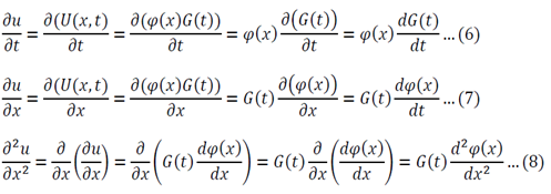
Substitute 6 and 8 into 1:

Function of only time = Function of only space

Both sides of the equation must equal to the same constant, called a separation constant. We get:

 

And

Equation 11 is the time depended equation and will be solved first. This is a first order linear homogeneous ODE and can be solved using the method of separation of variables.

The final solution will then be:

Analysis of possible values of lambda:

1. If lambda > 0 the temperature will exponentially decay with time
2. If lambda < 0 the temperature will exponentially increase with time
3. If lambda = 0 the temperature will stay constant

Only lambda => 0 makes sense as the temperature is not meant to grow to infinity.

Equation 12 is the space dependent equation. As equation 12 is a linear, second order, homogeneous ODE with constant coefficients, a method of constant coefficients can be used in order to solve that equation.

Substitution of 14 and 15 into 12 gives:

Equation 16 has numerous solutions, which all depend on the value of lambda:

Evaluate each of the cases

Lambda > 0

 

Lambda = 0

The solution of r=0 can be used here, or double integration can be used to solve equation 12

Substitution of equations 19, 20 and 13 into equation 5 gives the following general solution:

The boundary conditions now have to be applied:

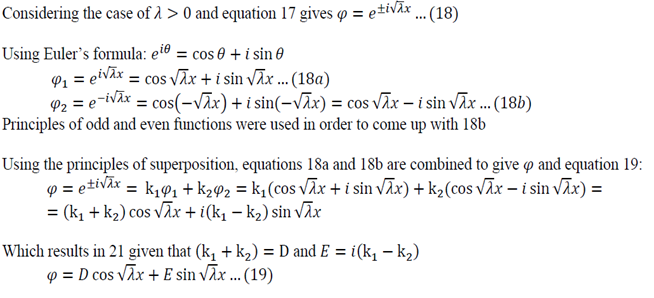
Lambda > 0

Using Equation 22 in 19:

Using Equation 23 in 19:

Solving Equation 24:

Lambda is now written with a subscript n as it could take on multiple values due to infinite number of possible solutions of the sin function.

Lambda = 0

Application of 22 in 20:

Application of 23 in 20:

So either L is zero or A is zero. Having zero length defeats the purpose of the problem so A = must be true.

Using all the values determined from the boundary conditions in equation 21:

Where C’ = CE

We now use the initial conditions and get:

So then:

We can apply the following identity:

Using equations 29 and 30, the left side of 31 becomes:

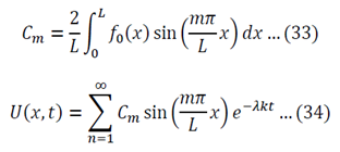
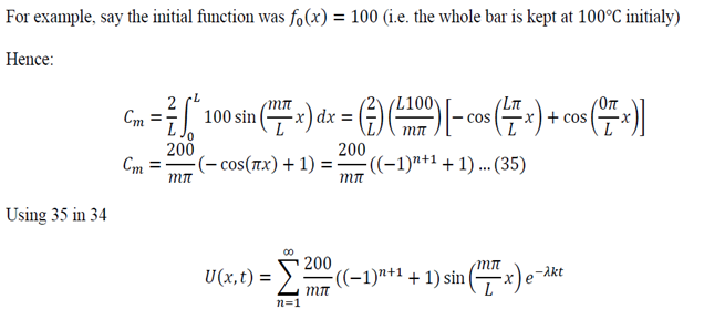
To generalize:

Technorati Tags: Differential Equations,Partial Differential Equations,Separation of Variables,Mathematics,Math Examples