Showing posts with label Examples. Show all posts

Thursday, April 30, 2009

Corrosion in a tank

One of the most common corrosion problems you will be asked to solve is how a tank, open to the atmosphere, corrodes and how you can control the rate of corrosion by simply covering the tank and regulating the pressure. Here is what is usually given:

T = 25oC

P = 1 atm

Corrosion Rate = 2.4 g Fe/cm2-yr

Say that O2 reduction is limited by mass transfer of dissolved O2 to the tank wall and the solubility of dissolved oxygen can be related to its partial pressure:

CO2 = 1.28x10⁻³ PO2

The partial pressure is in atm and the concentration is in mol/L. The oxidation of Feo is kinetically controlled in the Tafel region:

iO = 0.8x10⁻⁸ amp/cm2

Tafel Slope = 1/120 mV-1

ne = 1

Acceptable Corrosion Rate = 0.01 g Fe/cm2-yr

CFe2+ = 10-6 mol/L at all times

Feo -> Fe2+ + 2e-, -0.440 VSHE

And you are asked to determine the total pressure the headspace should be evacuated to to attain the acceptable corrosion rate.

Solution:

You are given that the O2 reduction is mass transfer limited so right away you can modify your general equation from:

clip_image002[11]

To:

clip_image004

From the given information you can find the concentration of dissolved oxygen in the bulk as well as the current from the Faraday’s law. Please see my earlier posts for more information on how to use Faraday’s to calculate current given a deposition rate.

clip_image006

From the given relationship between pressure and concentration, you can determine the bulk concentration of dissolved oxygen:

clip_image008

Now that you have all the required information, you can calculate the km value.

clip_image010

The next step is to determine the current density at the acceptable corrosion rate using the same line calculation as before:

clip_image012

Looking at the mass transfer limitation equation, we only have 1 unknown – the bulk concentration of dissolved oxygen, which is calculated via:

clip_image014

Great, now we can use the given relationship for partial pressure of oxygen and concentration to determine the partial pressure of oxygen in the headspace:

clip_image016

This is not the end, because oxygen only accounts for 21% of the composition of air, so the total headspace pressure has to be:

clip_image018

I apologize how bad some of the equations look. I really have to look into finding a new blog editor. If this has helped you in any way, please click on some of the ads.

Saturday, March 14, 2009

Partial Differential Equations – Separation of Variables


I received a great tutorial on how to apply separation of variables to solve a partial differential equation. I copied some of the equations as images because my generic editor cannot handle some symbols. The example is the following:

A uniform rod of length L with Finite Ends at Zero Temperature.

Equation given:

image

For 0 < x < L and t >= 0

Boundary Conditions:

  • U(0, t) = 0 … (2)
  • U(L,t) = 0 … (3)

Initial Conditions – U(x,o) = fo(x) … (4)

  • The PDE is linear and homogeneous
  • The boundary conditions are also linear and homogeneous

Separation of variables:

image

Adjust 5 so that it can be substituted into 1:

image

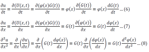
Substitute 6 and 8 into 1:

image

image

Function of only time = Function of only space

Both sides of the equation must equal to the same constant, called a separation constant. We get:

image 

And

image

Equation 11 is the time depended equation and will be solved first. This is a first order linear homogeneous ODE and can be solved using the method of separation of variables.

image

The final solution will then be:

image

Analysis of possible values of lambda:

  1. If lambda > 0 the temperature will exponentially decay with time
  2. If lambda < 0 the temperature will exponentially increase with time
  3. If lambda = 0 the temperature will stay constant

Only lambda => 0 makes sense as the temperature is not meant to grow to infinity.

Equation 12 is the space dependent equation. As equation 12 is a linear, second order, homogeneous ODE with constant coefficients, a method of constant coefficients can be used in order to solve that equation.

image

Substitution of 14 and 15 into 12 gives:

image

Equation 16 has numerous solutions, which all depend on the value of lambda:

image

Evaluate each of the cases

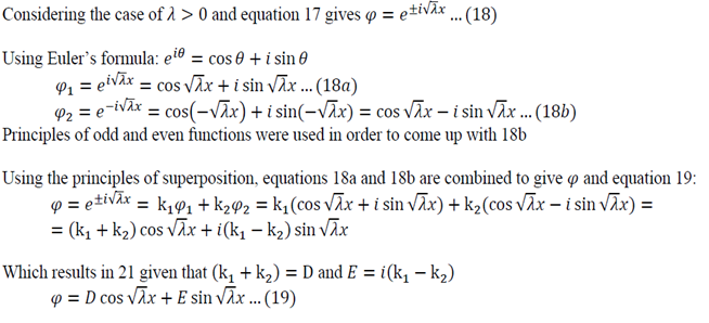
Lambda > 0

image 

Lambda = 0

The solution of r=0 can be used here, or double integration can be used to solve equation 12

image

Substitution of equations 19, 20 and 13 into equation 5 gives the following general solution:

image

The boundary conditions now have to be applied:

image

Lambda > 0

Using Equation 22 in 19:

image

Using Equation 23 in 19:

image

Solving Equation 24:

image

Lambda is now written with a subscript n as it could take on multiple values due to infinite number of possible solutions of the sin function.

Lambda = 0

Application of 22 in 20:

image

Application of 23 in 20:

image

So either L is zero or A is zero. Having zero length defeats the purpose of the problem so A = must be true.

Using all the values determined from the boundary conditions in equation 21:

image

Where C’ = CE

image

We now use the initial conditions and get:

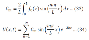
image

So then:

image

We can apply the following identity:

image

image

Using equations 29 and 30, the left side of 31 becomes:

image

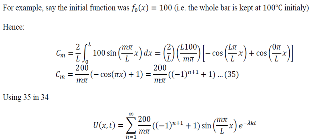
To generalize:

image

image